Project description

Little work in reinforcement learning studies of planning has formalized algorithms for backwards planning and their advantages over algorithms for forwards planning. Prior work in experimental psychology, however, has demonstrated humans have a general bias towards backwards planning (Park, Lu & Hedgcock, 2017, Psychological Science). The present study will investigate whether humans utilize an efficient form of backwards planning that we term a predecessor representation (PR). Like a successor representation (SR), a predecessor representation encodes long-run expectations of state occupancies given current states and actions taken. However, unlike a successor representation which predicts future state occupancies, a predecessor representation predicts past state occupancies. In the present study, we use simulations of the conditions under which PR-based planning would lead to better outcomes than SR-based planning or even more complex model-based (MB) planning, to develop a task to test whether individuals utilize PR-based planning. Below, I describe below pilot data (n=111) supporting our main hypothesis that individuals do indeed use PR-based planning, as well as the details of the planning task, our hypothesis, and the methods used to analyze the data we plan to collect. For the full details of our preregistration, see here: OSF Repository

.

Study design

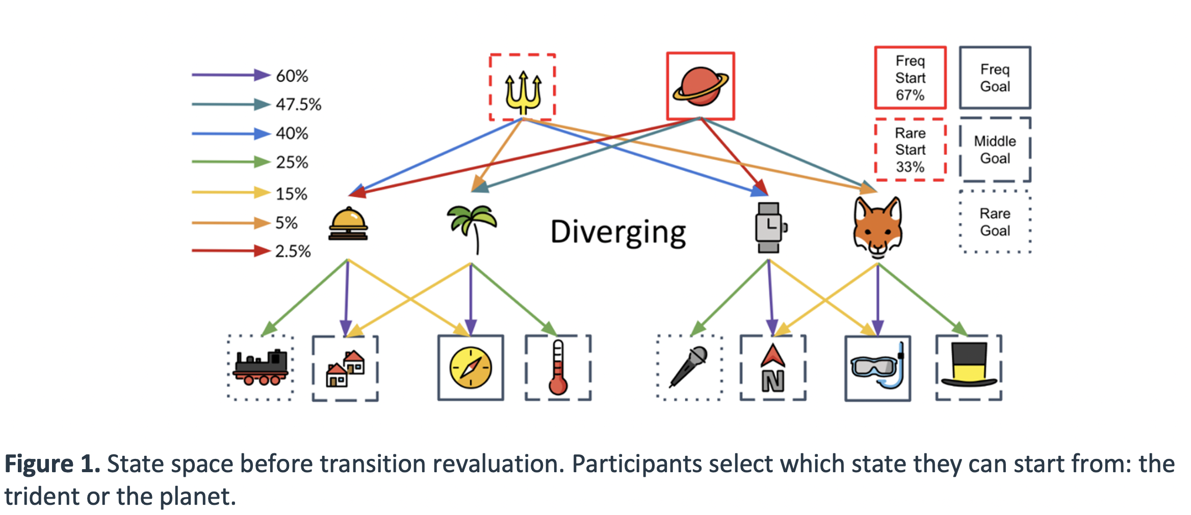
Task: Participants first complete 480 trials of a forced choice learning phase to ensure they know the state space and transitions well, and that each participant sample the same number of times from each state transition in the state space. Every 30 or so trials during this forced choice learning phase, participants are given a memory quiz where they must choose one of the two first-stage states that has the best chance of transitioning them to a 3rd stage state. We ensure in the piloting that our state space produced very good memory of the state space (average 93% on these memory probes).

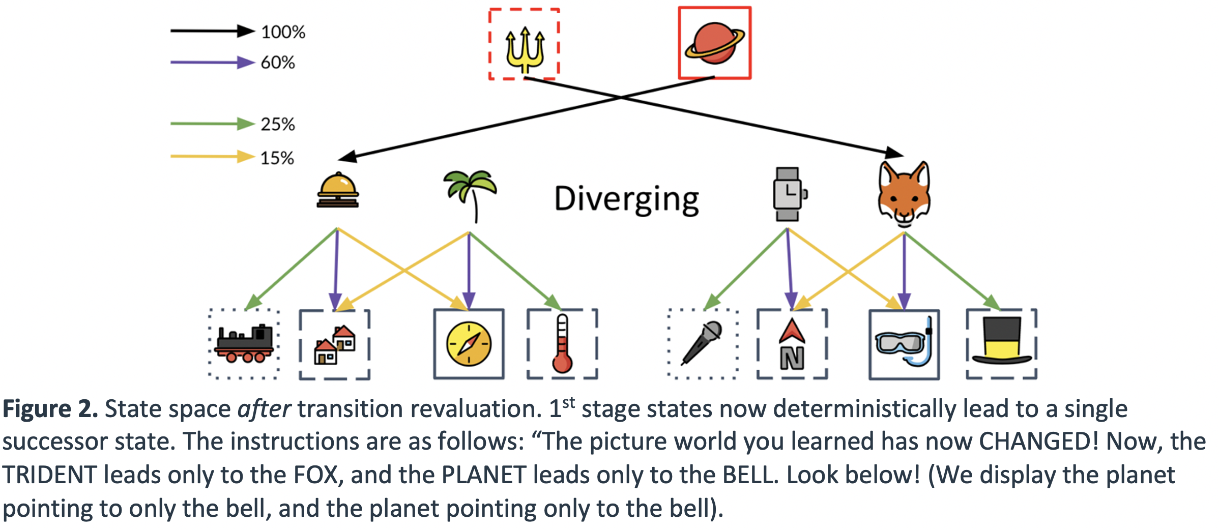
After this learning phase, participants face planning queries that ask them to use what they learned about the probability of transition to certain states in the preceding training phase to win the most money. We designed our task to specifically incentivize PR-based planning versus other forms of planning by hand-crafting specific planning queries that produce large action value differences between available choices according to PR-based planning, but no action value differences according to SR- or MB-based planning. We designed several additional sets of planning queries used to rule out confounding factors affecting participant behavior, which we delineate below:

1. Evidence participants utilize a PR vs. guessing (variable 1),
2. Evidence participants can perform transition revaluation using backwards-MB (variable 2)
3. Evidence participants have a bias for immediate vs. distal rewards when planning (variable 3)
4. Evidence participants can perform reward revaluation using any approximate (SR PR) strategy (variable 4)
5. Evidence participants have a bias to select the left or right action (variable 5).

.

Model of main hypothesis

Evidence of PR: We model the 8 choices participants made during planning queries comprising Variable 1 using a hierarchical beta-binomial model, that estimates the degree to which participants chose in line with PR-based planning predictions. A beta distribution at the group level defines the tendency of the group to choose in line with PR-based planning, which increases as the expected value of the beta distribution gets closer to 1. This group-level tendency is defined by its mode, and the spread of possible parameter values around the mode is captured by the distribution’s concentration. These central tendencies are recommended for beta distributions (Kruschke, 2014). In the hierarchical model, both the prior distribution of the group-level mode and concentration (i.e., the hyperpriors) are scaled to the data via BAMBI’s software default algorithm (Carpetto et al., 2020). At the subject-level, the binomial parameter is drawn from the group-level beta distribution, which defines the tendency of that individual to choose in line with PR-based planning. Finally, a binomial likelihood serves to account for the 8 choices each participant made.

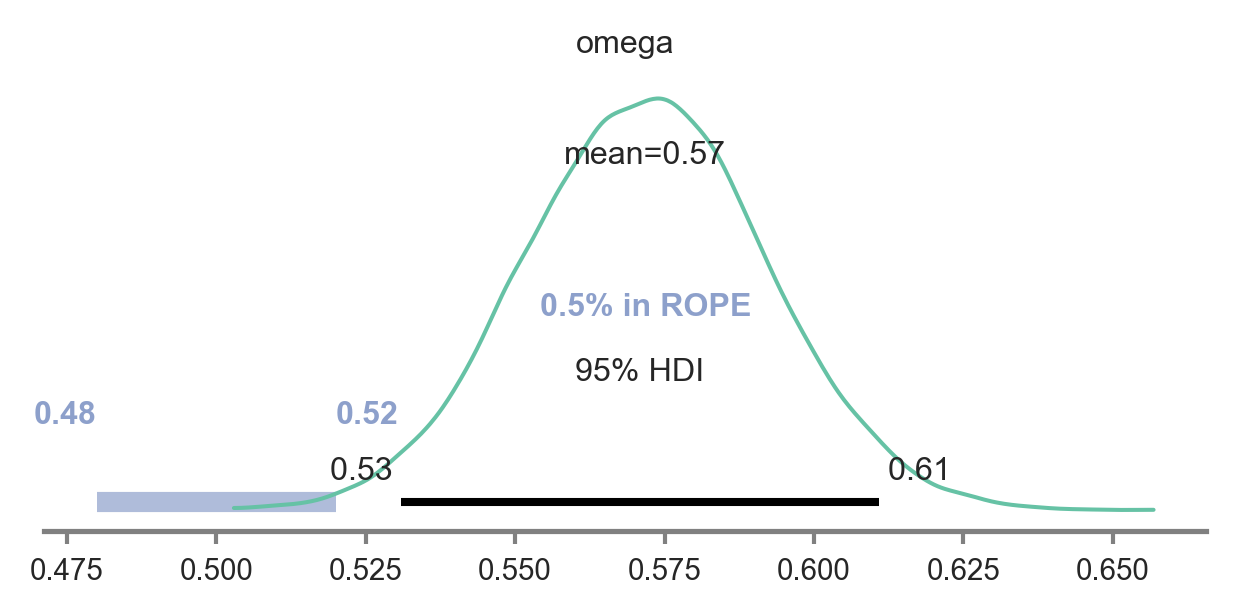
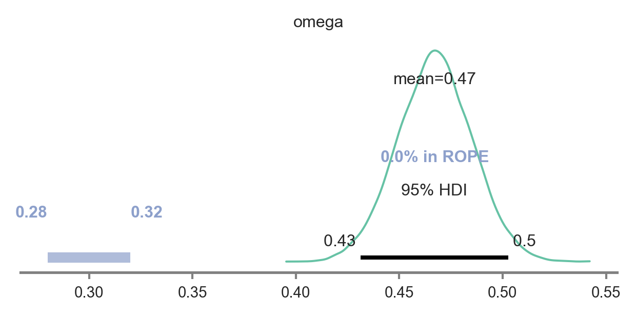
Below we fit the beta-binomial to choice data for Variable 1, which defines the number of times participants chose in line with PR-based planning. If omega, the mode of the group distribution, is estimated to be significantly greater than 0.5 (no evidence of PR-based planning), then we conclude evidence for our main hypothesis.

We followed Kruschke’s (2014) guidelines to derive the ROPE, wherein we took the standard deviation of the percentage of times subjects chose in line with PR-based planning and multiplied this value by 0.1 , which was 0.18, and multiplied this by 0.1, to define effects that are too small to be considered significant. We then rounded this up to 0.2 to make it even a bit more conservative than Kruschke’s (2014) recommendation. We use this ROPE for all subsequent analyses.

n_subjects = 111
subjects= [*range(111)]
with pm.Model() as hierarchical_model:
    omega = pm.Beta('omega', 1., 1.)
    kappa_minus2 = pm.Gamma('kappa_minus2', 1.105125 , 0.1051249, transform=None)
    kappa = pm.Deterministic('kappa', kappa_minus2 + 2)
    
    theta = pm.Beta('theta', alpha=omega*(kappa-2)+1, beta=(1-omega)*(kappa-2)+1, shape=n_subjects)

    y = pm.Binomial('y',n=8,p=theta[subjects], observed=PR_evidence) 
    
with hierarchical_model:
    trace_main = pm.sample(draws=4000, target_accept=0.99,init='adapt_diag')

Posterior distribution for group-level tendency to choose in line with PR-based planning

As you see below, the parameter omega defining the group-level tendency to choose in line with PR-based planning was significantly greater than the null value of 0.5. Specifically, the posterior highest density interval does not contain any values in the pre-defined region of practical equivalence, defining values similar-enough to 0.5 to be considered null effect sizes.

.

Fit model for manipulation check 1: Bias for distal reward?

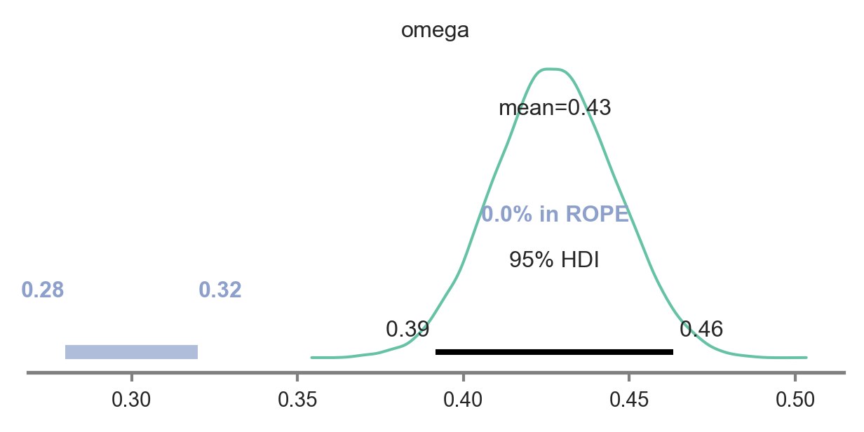
We fit the same beta-binomial hierarchical model described to model evidence for our main hypothesis to estimate the group-level tendency to display either a distal reward bias. The only difference in this model is that the choice data being modelled will come from Variable 3. As you see below, the manipulatin checked worked, as the posterior does not include 0.3.

.

Fit model for manipulation check 2: Bias for left-wards action?

We fit the same beta-binomial hierarchical model described to model evidence for our main hypothesis to estimate the group-level tendency to display a left-ward action bias. The only difference in this model is that the choice data being modelled will come from Variable 5. As you see below, the manipulatin checked worked, as the posterior does not include 0.3.

.

Fit model to determine if the cost of transition revaluation is significantly greater than the effect of reward evaluation

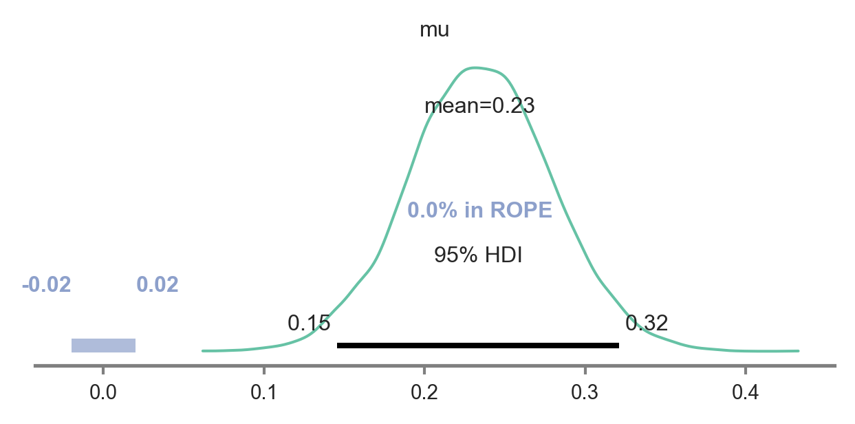
One additional test is necessary to support our main hypothesis, specifically, to show that there is only partial evidence of MB use, substantially less than what would be expected under the hypothesis that subjects only employ MB, implicating a hybrid use of backwards-MB and PR (similar to previous report of hybrid use of SR and forwards-MB; Momennejad et al., 2017). To test this, we examine whether the cost of transition revaluation (specifically, the difference between planning accuracy after transition revaluation and planning accuracy during the preceding reward revaluation), which MB agents can successfully handle, is greater than an upper bound estimate of the cost of reward revaluation (specifically, the difference between optimal planning accuracy – 100% – and planning accuracy during reward revaluation), which PR and MB agents can successfully handle.

We use a simple Bayesian model to estimate the mean of the difference between the cost of transition revaluation minus the cost of the reward revaluation, where this mean difference is drawn from a normal distribution with prior mean and variance on the scale of the data. As you can see in the posterior plot, there is a significantly greater cost to transition revaluation compared to reward revaluation.

from pymc3 import HalfCauchy, Model, Normal, glm, plot_posterior_predictive_glm, sample

subjects= [*range(111)]
with pm.Model() as model_effect_TR:  # model specifications in PyMC3 are wrapped in a with-statement
    # Define priors
    sigma = HalfCauchy("sigma", beta=10, testval=1.0)
    mu = Normal("mu", 0, sigma=20)

    # Define likelihood
    likelihood = Normal("y", mu=mu, sigma=sigma, observed=effect_TR)
    
with model_effect_TR:
    trace_effect_TR = pm.sample(draws=4000, target_accept=0.9999,init='adapt_diag')

.